


From Points to Hyperplanes – How Equations Shape Our Mathematical Universe
Introduction: The Hidden Geometry in Every Equation
Have you ever wondered why a simple equation like x + y = 5 represents a line? Or why adding more equations changes the shape of the solution from a plane to a line to a single point? The answer lies in one of mathematics’ most elegant principles: the relationship between equations and geometric dimensions.
In this comprehensive guide, you’ll discover the golden rule that governs how equations create geometric objects, understand why each equation reduces dimensionality, and see real-world applications that make these abstract concepts tangible and practical.
Whether you’re a student struggling with linear algebra, a teacher looking for clear explanations, or simply curious about mathematical beauty, this visual guide will transform how you see equations forever.
The Golden Rule: One Equation, One Dimension Lost
At the heart of understanding equations and geometry is this fundamental principle:
One equation with n unknowns creates an (n-1)-dimensional object
This simple formula unlocks everything. Let’s break it down with concrete examples.
Quick Reference: Equations to Geometric Objects
| Unknowns (n) | Space Dimension | Object Created | Example |
|---|---|---|---|
| 1 | 1D (number line) | Point (0D) | 2x = 6 → point at x = 3 |
| 2 | 2D (plane) | Line (1D) | x + y = 5 → line in plane |
| 3 | 3D (space) | Plane (2D) | x + y + z = 6 → plane in 3D |
| 4 | 4D | Hyperplane (3D) | x + y + z + w = 10 → 3D hyperplane |
Notice the pattern: each equation reduces the dimension by exactly one. This isn’t a coincidence – it’s a fundamental property of how constraints work in mathematics.
Visual progression: How equations reduce dimensions from 3D space to a single point

Why Does This Happen? The Constraint Perspective
Think of unknowns as dimensions of freedom – directions you can move. Each equation is a constraint that eliminates one of these freedoms.
A Real-World Example: Finding Your Location
Imagine you’re somewhere on Earth, which has three dimensions: latitude, longitude, and altitude. This is 3D space with infinite possibilities.
- No constraints: You could be anywhere on Earth – all of 3D space is available
- One constraint (equation): “You are at sea level” – Now you can only be on the 2D surface of the ocean
- Two constraints: “At sea level AND on the equator” – Now you can only move along the 1D line of the equator
- Three constraints: “Sea level, equator, AND prime meridian” – You’re locked to one 0D point off the coast of Africa
Each constraint removed one dimension of freedom, reducing the solution space from 3D → 2D → 1D → 0D.
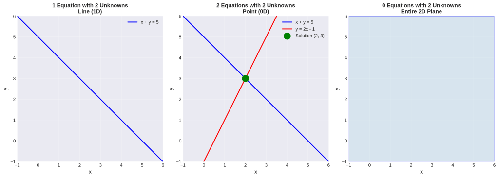
Examples of linear equations in 2D: entire plane, single line, and intersection point
Systems of Equations: The Intersection Principle
When you have multiple equations, each independent equation continues to reduce the dimension:
Solution Dimension = n – rank(A)
Where n is the number of unknowns and rank(A) is the number of independent (non-redundant) equations.
Two Unknowns: From Plane to Point
| Number of Equations | Rank | Solution Dimension | Geometric Shape |
|---|---|---|---|
| 0 | 0 | 2 | Entire 2D plane |
| 1 | 1 | 1 | A line |
| 2 | 2 | 0 | A point |
| 3+ | 2* | 0 or none | Point (if consistent) or no solution |
Note: Rank may be less than the number of equations if some equations are redundant (provide duplicate information).
Three Unknowns: From Space to Point
| Number of Equations | Rank | Solution Dimension | Geometric Shape |
|---|---|---|---|
| 0 | 0 | 3 | All of 3D space |
| 1 | 1 | 2 | A plane in 3D |
| 2 | 2 | 1 | A line in 3D |
| 3 | 3 | 0 | A point in 3D |
| 4+ | 3* | 0 or none | Point or no solution |
The golden rule visualized: How unknowns determine geometric object dimensions

Real-World Applications: Where Math Meets Reality
1. GPS and Navigation
Your GPS receiver determines your position by solving a system of equations:
- Each satellite provides one equation based on distance
- Three satellites give three equations → determines a unique point in 3D space
- Four satellites (including time correction) → pinpoint accuracy
2. Computer Graphics and 3D Modeling
When rendering 3D graphics:
- Planes (one equation) define surfaces like walls or screens
- Lines (two equations) represent edges where surfaces meet
- Points (three equations) mark vertices and intersections
3. Chemistry and Material Science
Mixing solutions with constraints:
- Total volume = 1 liter (one equation) → 2D plane of possible mixtures
- Concentration = 30% (second equation) → 1D line of solutions
- pH = 7.0 (third equation) → unique 0D point solution
4. Economics and Resource Allocation
Budget constraints in economics work exactly like geometric equations. If you have three products to buy (three unknowns), each budget constraint or requirement is an equation that limits your choices, reducing the solution space from 3D to 2D to 1D to a single optimal point.
Special Cases: When Systems Behave Differently
Underdetermined Systems (Fewer Equations Than Unknowns)
Example: 2 equations with 3 unknowns → Solution is a line (1D) with infinite points
These systems have infinitely many solutions because you haven’t constrained enough dimensions. It’s like asking someone to meet you “on Main Street” without specifying where – there are infinite possible meeting points along that street.
Exactly Determined Systems (Equal Equations and Unknowns)
Example: 3 equations with 3 unknowns → Usually one unique solution (a point)
This is the ideal case in many applications. You have just enough information to determine a unique answer, like having exactly the right number of GPS satellites to pinpoint your location.
Overdetermined Systems (More Equations Than Unknowns)
Example: 4 equations with 2 unknowns → Often no exact solution
These systems are usually inconsistent. It’s like trying to be in two places at once – the constraints contradict each other. In practice, we often find the “best fit” solution that comes closest to satisfying all equations.
Redundant Equations: The Hidden Trap
Not all equations add new constraints. If two equations say the same thing in different ways (like “x + y = 5” and “2x + 2y = 10”), the second equation is redundant. The rank of the system tells you how many truly independent constraints you have.
Visual Understanding: Seeing the Dimensions
The Corner Analogy
Imagine standing in a room (3D space):
- No walls: Free movement in all directions (3D)
- One wall: Can move along the wall’s surface (2D plane)
- Two walls (corner edge): Can only move up/down the edge (1D line)
- Three walls (corner point): Stuck at the corner (0D point)
Each wall is an equation, each position where walls meet represents a lower-dimensional solution.
Practical Tips for Students and Educators
For Students
- Count your unknowns first: This tells you the dimension of the space you’re working in
- Count independent equations: Each one reduces the dimension by 1
- Subtract: Dimension of solution = unknowns – independent equations
- Visualize: Try to imagine the geometric object in lower dimensions (2D or 3D) before working with higher dimensions
For Educators
- Start with 2D examples: Students can easily visualize lines and points on paper
- Use physical demonstrations: Room corners, maps, and location finding are tangible
- Emphasize the constraint perspective: Help students see equations as limitations on freedom
- Connect to real applications: GPS, graphics, and chemistry make the math meaningful
Quick Reference Card
| Concept | Formula/Rule |
|---|---|
| Single equation dimension | Object dimension = n – 1 |
| System solution dimension | Solution dimension = n – rank(A) |
| Constraint effect | Each independent equation reduces dimension by 1 |
| Underdetermined | More unknowns than equations → infinite solutions |
| Exactly determined | Equal unknowns and equations → usually one solution |
| Overdetermined | More equations than unknowns → usually no solution |
Conclusion: The Beauty of Mathematical Structure
The relationship between equations and geometry reveals one of mathematics’ most elegant truths: abstract algebraic constraints directly correspond to concrete geometric shapes. Every equation is a window into a lower-dimensional world, and systems of equations are intersections where these worlds meet.
Whether you’re navigating with GPS, rendering 3D graphics, optimizing a budget, or simply solving homework problems, you’re participating in this beautiful mathematical dance between constraints and freedom, equations and geometry, algebra and space.
The next time you see an equation, don’t just see symbols on paper. See the geometric object it creates, the dimension it inhabits, and the constraints it represents. That’s the true power of mathematical thinking.
I hope this tutorial will create a good foundation for you. If you want tutorials on another topic or you have any queries, please send an mail at contact@spatial-dev.guru.