A practical GIS and AI workflow for terrain-aware telecom coverage simulation and tower-selection optimization.

Introduction

Planning a wireless network is not just about placing towers on a map. A tower that looks well-positioned in 2D may perform poorly in the real world because hills, valleys, distance, antenna height, and terrain obstruction all affect signal propagation.

The core question is simple:

From a large set of possible tower locations, how can we select the smallest number of towers that still covers the maximum possible area?

This problem becomes difficult very quickly. If there are hundreds of candidate towers, testing every possible combination is not practical. Each tower may cover a different area, many towers overlap, and some towers may contribute very little additional coverage. This makes the problem a classic combinatorial optimization challenge.

In this project, I built a complete geospatial workflow for 4G/5G-style coverage optimization. The workflow starts with terrain data, simulates wireless coverage for candidate tower locations, converts raster coverage into a grid-based optimization dataset, and then uses a Genetic Algorithm to select an efficient tower subset.

The goal was not only to simulate coverage, but to answer a more useful planning question: Which towers should be selected when the objective is high coverage with fewer towers?

Why Tower Coverage Optimization Is Hard

Wireless tower planning looks simple at first: place towers at high points and spread them across the area. But in practice, several factors make this difficult:

• Terrain blocks radio signals.
• Towers may overlap heavily in some areas.
• Some remote regions may require many towers for small coverage gains.
• Higher coverage targets usually require disproportionately more towers.
• The best local decision does not always produce the best network-wide solution.

For example, one tower may cover a large visible region, but if that region is already covered by other towers, its additional value is low. Another tower may cover a smaller area, but that area may be completely uncovered by the rest of the network. This is why simple ranking by individual coverage is not enough.

The problem must be solved at the system level, where every selected tower is evaluated based on how much unique coverage it adds to the final network.

Step 1: Start with Terrain Data

The first input was a Digital Elevation Model, or DEM. A DEM is a raster dataset where each pixel stores an elevation value. Lower values usually represent valleys, while higher values represent ridges, hills, or peaks.

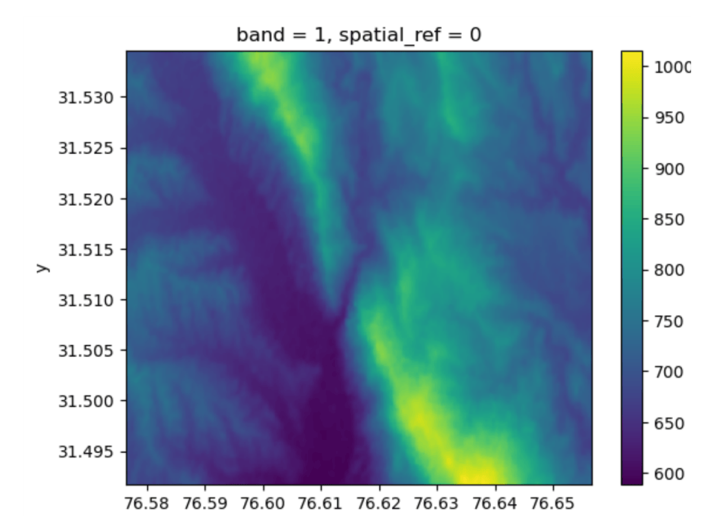
Figure 1. Digital Elevation Model showing terrain height variation

The DEM is important because wireless coverage depends strongly on line of sight. A tower placed behind a ridge may not serve the valley on the other side, even if the horizontal distance is small.

To better understand the terrain, the DEM was also visualized in 3D. This makes it easier to see ridges, valleys, slope direction, and high-elevation zones that may be suitable for candidate tower placement.

Figure 2. 3D terrain visualization generated from the DEM

In mountainous regions, this terrain-first approach is critical. A flat-distance model alone would overestimate coverage because it would ignore physical obstruction.

Step 2: Generate Candidate Tower Locations

After preparing the DEM, the next step was to generate possible tower locations. Since the goal was simulation and optimization, the workflow needed a structured way to create many candidate sites.

A grid-based approach was used:

1. Divide the terrain into regular grid cells.

2. Inspect elevation values inside each grid cell.

3. Select high-elevation points as candidate tower locations.

4. Use those candidate points for line-of-sight and coverage simulation.

Figure 3. Candidate tower locations selected using a grid-based terrain approach

This approach gives a reasonable first-pass candidate set because higher terrain usually improves visibility. It also avoids placing all candidate towers in one dense cluster by forcing the search to consider the entire geographic extent.

This does not mean every high point is automatically a good tower. It only creates a candidate pool. The optimization algorithm later decides which of these candidates are actually worth selecting.

Step 3: Perform Line-of-Sight Analysis

For every candidate tower, a line-of-sight analysis was generated using the DEM. We have used GDAL’s vieshed utility for performing line of sight analysis. The purpose was to identify which pixels are visible from the tower location.

The result is a binary visibility raster:

• Visible pixels are potential service areas.
• Non-visible pixels are blocked by terrain.

Figure 4. Line-of-sight viewshed raster for a candidate tower location

This step is important because radio signal should not be modeled only as a circular buffer. A circular buffer assumes that signal spreads equally in all directions, but terrain does not allow that in hilly regions. The viewshed layer acts as a terrain-aware mask, limiting the simulated signal to areas that are actually visible from the tower.

In simple terms:

The tower may have enough power to reach a location, but if the terrain blocks the path, that location should not be treated as covered.

Step 4: Simulate Signal Strength Using Path Loss

Once the visible area was known, signal strength was simulated using a Free Space Path Loss model and RSSI calculation.

The Free Space Path Loss formula estimates how much signal power is lost as the signal travels through space:

FSPL(dB) = 20 * log10(4 * pi * d / lambda)

Where:

• d is the distance between transmitter and receiver.
• lambda is the signal wavelength.
• lambda = c / f, where c is the speed of light and f is frequency.

The received signal strength was then estimated using:

RSSI = Transmit Power + Transmitter Antenna Gain + Receiver Antenna Gain – Path Loss – Cable Loss

The output is a raster where each pixel stores estimated signal strength. Stronger pixels are closer to the tower or have better propagation conditions. No-signal pixels remain excluded.

Figure 5. Single tower signal strength simulation after visibility and path loss modeling

This is still a simplified model. Real-world 4G/5G planning also considers buildings, vegetation, diffraction, reflection, clutter classes, antenna tilt, bandwidth, capacity, interference, and user demand. However, for a terrain-driven optimization experiment, this provides a strong foundation.

Step 5: Build Coverage Rasters for All Candidate Towers

The same process was repeated for each candidate tower:

1. Calculate visible pixels using terrain.

2. Estimate distance from tower to visible pixels.

3. Apply path loss.

4. Calculate RSSI.

5. Store the result as a georeferenced coverage raster.

After processing many tower candidates, the combined coverage surface starts to show which parts of the terrain are easier to cover and which regions remain difficult.

Figure 6. Combined wireless coverage simulation from multiple candidate towers

At this stage, the project moves from geospatial simulation to optimization. The raw raster data is useful visually, but optimization requires a structured table that an algorithm can evaluate efficiently.

Step 6: Convert Raster Coverage into Grid-Based Data

To prepare the optimization dataset, the coverage rasters were converted into a grid-based summary.

Each grid cell represents a geographic area. For each tower and grid cell, the workflow calculates how many covered pixels fall inside that grid.

The final optimization table follows this structure:

Field	Meaning
TowerID	Unique identifier of the candidate tower
GridID	Unique identifier of the grid cell
NumPixel	Number of covered pixels contributed by that tower inside the grid

This table is much easier to use in optimization than raw rasters. Instead of reading large images repeatedly, the algorithm can evaluate tower combinations using grid-level coverage counts.

Figure 7. Grid-based coverage representation used for optimization

The grid also helps reduce complexity. Rather than optimizing at individual pixel level, the algorithm works with meaningful spatial units. This improves performance while still preserving the geographic distribution of coverage.

Step 7: Formulate the Optimization Problem

The optimization problem can be expressed as:

Select the minimum number of towers that covers the maximum number of grid cells or pixels.

Each tower can be represented as a binary decision:

1 = tower selected

0 = tower not selected

For 648 candidate towers, a solution is a binary vector of length 648. For example:

[1, 0, 0, 1, 1, 0, …]

This means some towers are selected and others are ignored. The algorithm must search through many such combinations and find the best trade-off between coverage and tower count.

A useful fitness function must reward coverage and penalize unnecessary towers. A simplified objective can be written as:

Cost = w1 * Number of Selected Towers + w2 * Uncovered Area

The algorithm then tries to minimize this cost.

The balance between w1 and w2 controls the behavior:

• Higher tower penalty selects fewer towers but may leave more uncovered area.
• Higher uncovered-area penalty improves coverage but usually selects more towers.

This trade-off is the heart of telecom coverage optimization.

Step 8: Use a Genetic Algorithm for Tower Selection

A Genetic Algorithm was used to search for a good tower subset. Genetic Algorithms are useful when the search space is too large for brute force and when the goal is to find a strong near-optimal solution.

The Genetic Algorithm follows this process:

1. Create an initial population of random tower combinations.

2. Evaluate each combination using the fitness function.

3. Select better-performing combinations as parents.

4. Apply crossover to mix parent solutions.

5. Apply mutation to introduce variation.

6. Repeat for many generations.

7. Keep the best tower combination found.

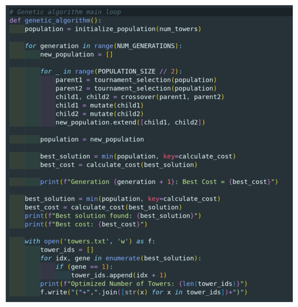
Figure 8. Genetic Algorithm main loop used for tower selection

The main advantage of a Genetic Algorithm is that it searches globally. It does not simply pick the biggest tower coverage one by one. Instead, it evaluates combinations, which is important when tower coverage overlaps.

Result: Fewer Towers with High Coverage

In the simulation, the Genetic Algorithm selected 347 towers out of 648 candidate towers while covering more than 85% of the target area.

With parameter tuning, it was possible to push coverage above 90%, but this required around 400 towers. That result clearly shows the trade-off between infrastructure cost and coverage quality.

The important insight is not just the final number. The real value is the decision-support workflow:

• Simulate candidate coverage using terrain.
• Convert coverage into optimization-ready grid data.
• Use AI-style search to identify efficient tower combinations.
• Compare different coverage targets and tower-count trade-offs.

This gives planners a practical way to ask questions such as:

• How many towers are needed for 80%, 85%, or 90% coverage?
• Which towers provide the most unique coverage?
• Where are the persistent coverage gaps?
• How much additional infrastructure is needed for marginal coverage improvement?

Key Learnings

The biggest lesson from this workflow is that telecom coverage optimization is not a single-step mapping problem. It is a pipeline that combines terrain modeling, signal simulation, raster processing, tabular aggregation, and algorithmic search.

A few important observations stood out:

1. Terrain matters a lot

In hilly regions, line of sight can completely change the expected coverage pattern. A simple circular buffer would produce misleading results.

2. Raster data must be converted for optimization

Coverage rasters are excellent for visualization, but optimization works better with structured grid-level summaries.

3. The best tower is not always the tower with the largest individual coverage

A tower is valuable only if it adds unique coverage that other towers do not already provide.

4. Coverage and cost are always in tension

Reaching the last 10-15% of coverage may require a large number of additional towers, especially in difficult terrain.

5. Metaheuristic optimization is practical for large candidate sets

A Genetic Algorithm can produce strong solutions without checking every possible tower combination.

Limitations

This workflow is a strong prototype, but it can be improved further for production-grade telecom planning.

Some limitations include:

• The path loss model is simplified.
• Buildings, vegetation, and land-cover clutter are not fully modeled.
• Interference between towers is not considered.
• Capacity and user demand are not included.
• Antenna orientation, tilt, and sectorization are not deeply modeled.
• Genetic Algorithm performance depends on parameter tuning.
• Larger study areas may require parallel processing or distributed computation.

These limitations are expected in a simulation-first workflow. The value of the project is that it creates an extensible foundation where more realistic RF models and constraints can be added later.

Future Improvements

Several improvements can make this workflow more realistic and scalable:

• Use more advanced propagation models for different environments.
• Add clutter data such as buildings, vegetation, and land use.
• Include antenna azimuth, beam width, tilt, and sector-level coverage.
• Add capacity and population demand layers.
• Use multi-objective optimization for coverage, cost, capacity, and redundancy.
• Compare Genetic Algorithm results with Particle Swarm Optimization, Ant Colony Optimization, and Simulated Annealing.
• Parallelize raster processing for thousands of candidate towers.
• Build an interactive dashboard for planners to explore tower trade-offs visually.

Conclusion

This project demonstrates how GIS and AI-style optimization can be combined for telecom network planning. The workflow starts with terrain, simulates line-of-sight and signal strength, transforms raster coverage into grid-based data, and then uses a Genetic Algorithm to select an efficient subset of towers.

The final result showed that it was possible to cover more than 85% of the target area using 347 towers out of 648 candidates. Increasing the target coverage above 90% required more towers, highlighting the practical trade-off between coverage and infrastructure cost.

For telecom GIS teams, this type of workflow can act as a decision-support system. It helps planners move beyond manual tower selection and toward data-driven, terrain-aware, optimization-based network design.

---

I hope this tutorial will create a good foundation for you. If you want tutorials on another GIS topic or you have any queries, please send an mail at contact@spatial-dev.guru.